using Yao, BitBasis
using NLopt

include("maxcut_gw.jl")

"""
Transverse field term
"""
HB(nbit::Int) = sum([put(nbit, i=>X) for i=1:nbit])

"""
Target Hamiltonian.
"""
function HC(W::AbstractMatrix)
    nbit = size(W, 1)
    ab = Any[]
    for i=1:nbit,j=i+1:nbit
        if W[i,j] != 0
            push!(ab, 0.5*W[i,j]*repeat(nbit, Z, [i,j]))
        end
    end
    sum(ab)
end

julia> TimeEvolution(HB(3), 0.1)
Time Evolution Total: 3, DataType: Complex{Float64}
+
├─ put on (1)
│  └─ X gate
├─ put on (2)
│  └─ X gate
└─ put on (3)
   └─ X gate
Δt = 0.1, tol = 1.0e-7

julia> W = [0 1 3; 1 0 1; 3 1 0]   # 3x3 的全连接图
3×3 Array{Int64,2}:
 0  1  3
 1  0  1
 3  1  0

julia> hc = HC(W)
Total: 3, DataType: Complex{Float64}
+
├─ [0.5] repeat on (1, 2)
│  └─ Z gate
├─ [1.5] repeat on (1, 3)
│  └─ Z gate
└─ [0.5] repeat on (2, 3)
   └─ Z gate

julia> ishermitian(hc)
true

function qaoa_circuit(W::AbstractMatrix, depth::Int; use_cache::Bool=false)
    nbit = size(W, 1)
    hb = HB(nbit)
    hc = HC(W)
    use_cache && (hb = hb |> cache; hc = hc |> cache)
    c = chain(nbit, [repeat(nbit, H, 1:nbit)])
    append!(c, [chain(nbit, [time_evolve(hc, 0.0, tol=1e-5),
                        time_evolve(hb, 0.0, tol=1e-5)]) for i=1:depth])
end

julia> qaoa_circuit(W, 2)
Total: 3, DataType: Complex{Float64}
chain
├─ repeat on (1, 2, 3)
│  └─ H gate
├─ chain
│  ├─ Time Evolution Total: 3, DataType: Complex{Float64}
│  │  +
│  │  ├─ [0.5] repeat on (1, 2)
│  │  │  └─ Z gate
│  │  ├─ [1.5] repeat on (1, 3)
│  │  │  └─ Z gate
│  │  └─ [0.5] repeat on (2, 3)
│  │     └─ Z gate
│  │  Δt = 0.0, tol = 1.0e-5
│  └─ Time Evolution Total: 3, DataType: Complex{Float64}
│     +
│     ├─ put on (1)
│     │  └─ X gate
│     ├─ put on (2)
│     │  └─ X gate
│     └─ put on (3)
│        └─ X gate
│     Δt = 0.0, tol = 1.0e-5
└─ chain
   ├─ Time Evolution Total: 3, DataType: Complex{Float64}
   │  +
   │  ├─ [0.5] repeat on (1, 2)
   │  │  └─ Z gate
   │  ├─ [1.5] repeat on (1, 3)
   │  │  └─ Z gate
   │  └─ [0.5] repeat on (2, 3)
   │     └─ Z gate
   │  Δt = 0.0, tol = 1.0e-5
   └─ Time Evolution Total: 3, DataType: Complex{Float64}
      +
      ├─ put on (1)
      │  └─ X gate
      ├─ put on (2)
      │  └─ X gate
      └─ put on (3)
         └─ X gate
      Δt = 0.0, tol = 1.0e-5

function cobyla_optimize(circuit::MatrixBlock{N}, hc::MatrixBlock; niter::Int) where N
    function f(params, grad)
        reg = zero_state(N) |> dispatch!(circuit, params)
        loss = expect(hc, reg) |> real
        #println(loss)
        loss
    end
    opt = Opt(:LN_COBYLA, nparameters(circuit))
    min_objective!(opt, f)
    maxeval!(opt, niter)
    cost, params, info = optimize(opt, parameters(circuit))
    pl = zero_state(N) |> circuit |> probs
    cost, params, pl
end

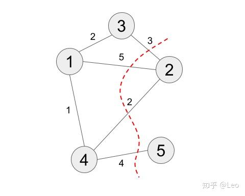
nbit = 5
W = [0 5 2 1 0;
	 5 0 3 2 0;
	 2 3 0 0 0;
	 1 2 0 0 4;
	 0 0 0 4 0]

# the exact solution
exact_cost, sets = goemansWilliamson(W)

hc = HC(W)
# the cut is -<Hc> + sum(wij)/2
@test -expect(hc, product_state(5, bmask(sets[1]...)))+sum(W)/4 ≈ exact_cost

# build a QAOA circuit and start training.
qc = qaoa_circuit(W, 20; use_cache=false)
opt_pl = nothing
opt_cost = Inf
for i = 1:10
	dispatch!(qc, :random)
	cost, params, pl = cobyla_optimize(qc, hc; niter=2000)
	@show cost
	cost < opt_cost && (opt_pl = pl)
end

cost=-5.056439885146659
cost=-5.3148313277163455
cost=-5.314515402351343
cost=-5.27061216619153
cost=-5.218577446603341
cost=-5.140030583281352
cost=-4.859469398853606
cost=-5.445797991390686
cost=-5.2074338799039
cost=-4.971171116896116

# check the correctness of result
config = argmax(opt_pl)-1
@test config in [bmask(set...) for set in sets]

using Convex
using SCS
using LinearAlgebra

"
The Goemans-Williamson algorithm for the MAXCUT problem.

Adapted From: https://github.com/ericproffitt/MaxCut
"

function goemansWilliamson(W::Matrix{T}; tol::Real=1e-1, iter::Int=100) where T<:Real
	"Partition a graph into two disjoint sets such that the sum of the edge weights
	which cross the partition is as large as possible (known to be NP-hard)."

	"A cut of a graph can be produced by assigning either 1 or -1 to each vertex.  The Goemans-Williamson
	algorithm relaxes this binary condition to allow for vector assignments drawn from the (n-1)-sphere
	(choosing an n-1 dimensional space will ensure seperability).  This relaxation can then be written as
	an SDP.  Once the optimal vector assignments are found, origin centered hyperplanes are generated and
	their corresponding cuts evaluated.  After 'iter' trials, or when the desired tolerance is reached,
	the hyperplane with the highest corresponding binary cut is used to partition the vertices."

	"W:		Adjacency matrix."
	"tol:	Maximum acceptable distance between a cut and the MAXCUT upper bound."
	"iter:	Maximum number of hyperplane iterations before a cut is chosen."

	LinearAlgebra.checksquare(W)
	@assert LinearAlgebra.issymmetric(W)	"Adjacency matrix must be symmetric."
	@assert all(W .>= 0)			"Entries of the adjacency matrix must be nonnegative."
	@assert all(diag(W) .== 0)		"Diagonal entries of adjacency matrix must be zero."
	@assert tol > 0					"The tolerance 'tol' must be positive."
	@assert iter > 0				"The number of iterations 'iter' must be a positive integer."

	"This is the standard SDP Relaxation of the MAXCUT problem, a reference can be found at
	http://www.sfu.ca/~mdevos/notes/semidef/GW.pdf."
	k = size(W, 1)
	S = Semidefinite(k)

	expr = dot(W, S)
	constr = [S[i,i] == 1.0 for i in 1:k]
	problem = minimize(expr, constr...)
	solve!(problem, SCSSolver(verbose=0))

	### Ensure symmetric positive-definite.
	A = 0.5 * (S.value + S.value')
	A += (max(0, -eigmin(A)) + eps(1e3))*I

	X = Matrix(cholesky(A))

	### A non-trivial upper bound on MAXCUT.
	upperbound = (sum(W) - dot(W, S.value)) / 4

	"Random origin-centered hyperplanes, generated to produce partitions of the graph."
	maxcut = 0
	maxpartition = nothing

	for i in 1:iter
		gweval = X' * randn(k)
		partition = (findall(x->x>0, gweval), findall(x->x<0, gweval))
		cut = sum(W[partition...])

		if cut > maxcut
			maxpartition = partition
			maxcut = cut
		end

		upperbound - maxcut < tol && break
		i == iter && println("Max iterations reached.")
	end
	return round(maxcut; digits=3), maxpartition
end

using Test
@testset "max cut" begin
	W = [0 5 2 1 0;
		 5 0 3 2 0;
		 2 3 0 0 0;
		 1 2 0 0 4;
		 0 0 0 4 0]

	maxcut, maxpartition = goemansWilliamson(W)
	@test maxcut == 14
	@test [2,5] in maxpartition
end